|
The functions that we have seen so far have been expressed
as a single equation.
We are now going to take a look at functions
that are a combination of two, or more, equations.
These will be functions made up of "pieces"
(with each "piece" being a separate equation). |
 |
When working with real world situations, it may be necessary to graph more than one function equation to represent the conditions in one problem. These multiple function "pieces" often arise when two or more differing rates occur over the duration of one problem.
So, how do we graph equations as "pieces"?
 |
A piecewise-defined function is a function which uses a combination of equations over the intervals of its domain.
(Also called a piecewise function, or a split-definition function.) |
|
Remember, the domain is the set of all possible x-coordinates used to create a graph.
The set of all of the y-coordinates used by these
domain elements is called the range.
Each equation (or "piece") of a piecewise function will have restrictions placed on its domain.
 Note: The domain for an entire piecewise-defined graph will be Note: The domain for an entire piecewise-defined graph will be
the union of the restricted domains for each piece.
The "pieces" that make up a piecewise-defined functions may be of varying types
(linear, quadratic, exponential, etc.),
or a combination of types.
On this page, we are going to examine only piecewise functions
whose "pieces" are linear equations. |
When graphing functions, remember that y = f (x), allowing for either "y" or "f (x)" to represent the function.
Graphing a linear piecewise-defined function:
Since we know this is a "linear" piecewise function, we know that the graphs will be composed of line segments and/or rays.
Method 1: Plot points within the restricted domains for each "piece".
• If the restricted domain indicates a line segment (such as 2 < x < 8), plot each end point and draw the segment using open and/or closed circles as indicated by the domain.
• If the restricted domain indicates a ray (such as x < 4), plot the end point using an open/closed circle as indicated. Then plot another point within the restriction and draw the ray.
Method 2: Graph lines using slope-intercept method (y = mx + b) for each "piece".
• Graph an entire line for each "piece" using a faint dashed line. Then draw solid markings on each line to indicated the restrictions. (This can get to be a bit messy.) |

 Graphing a Linear Piecewise Function Given its Definition: Graphing a Linear Piecewise Function Given its Definition: |
Notice the domain restrictions placed on each equation "piece".
Graph the function defined as:
To graph Part 1: Choose the endpoints from the restricted domain and plug into y = 2x + 1.
For x = -2, we get y = -3.
Plot (-2,-3) with closed circle.
For x = 2, we get y = 5. Plot (2,5) with open circle.
To graph Part 2: Choose the endpoints from the restricted domain and plug into y = x - 1.
For x = 2, we get y = 1.
Plot (2,1) with closed circle.
For x = 5, we get y = 4. Plot (5,4) with closed circle.
The linear equations in this problem tell us we have two linear segments. The completed graph will start at x = -2 and stop at x = 5, with all values between being used. The domain of the entire function is [-2,5].
|
Piecewise-defined Function
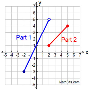
Domain for function y: -2 < x < 5 or [-2.5]
Range for function y: -3 < y < 5 or [-3,5)
Both segments in this graph
are increasing
across
their restricted domains.
|
In this example, the two "pieces" of the graph are NOT joined together, so the graph is described as being "discontinuous" since there is a "break" in the graph. For a function to be "continuous"over an interval, you must be able to draw the graph without taking your pencil off the paper (no breaks).
In addition, the graph is a "function", since any vertical line drawn in the interval from -2 to 5 will intersect the graph only once. Notice at x = 2 that we have an open circle and a closed circle, allowing for a vertical line to intersect only the Part 2 section of the graph.
|
| NOTE: In this graph at x = 2, the red endpoint at (2,1) is closed (shaded), but the blue endpoint at (2,5) is open (not shaded). If the blue endpoint had been shaded, this graph would no longer be a function. Functions only allow for ONE y-value to be assigned to each x-value. |
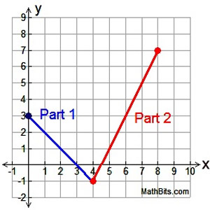
Let's see a graph where the "parts" are connected.
Graph the function defined as:
This function consists of two linear segments. The completed graph will start at x = 0 and stop at x = 8.
Its entire domain will be the interval [0,8], all values between 0 and 8 inclusive.
Part 1: Using the restricted domain's endpoints (0 & 4)
and y = -x + 3, we plot (0,3) with a closed circle,
and plot (4, -1) with an open circle.
Part 2: Using the restricted domain's endpoints (4 & 8)
and y = 2x - 9, we plot (4,-1) with a closed circle,
and plot (8, 7) with a closed circle.
|
Piecewise-defined Function
Domain for function y: 0 < x < 8 or [0, 8]
Range for function y: -1 < y < 7 or [-1, 7]:
Part 1 is decreasing.
Part 2 in increasing.
|
In this example, the two "parts" of the graph are joined together at the point (4,-1).
The point (4,-1) belongs to Part 2. The point (4,-1) is "approached" by Part 1 from the left, but does not "belong" to Part 1.
If you could see just the graph of Part 1, you would see an open circle at (4,-1).
Unlike the previous example, this graph (over its domain) is "continuous". The graph can be drawn over the entire domain without removing your pencil from your paper.
In addition, the Vertical Line Test is upheld across this graph proving that we are working with a function. |
Let's see a graph with "rays" instead of "segments".
Graph the function defined as:
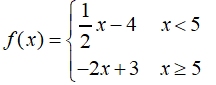
To graph Part 1: Using y = mx + b, the slope m = ½ and the y-intercept, b = -4, draw dashed line. Mark off restrictions on the line with a solid drawing.
To graph Part 2: Using y = mx + b, the slope m = -2 and the y-intercept, b = 3, draw dashed line. Mark off restrictions on the line with a solid drawing.
In this example, we are dealing with "pieces" that are two "rays" instead of two line segments.
|
Piecewise-defined Function
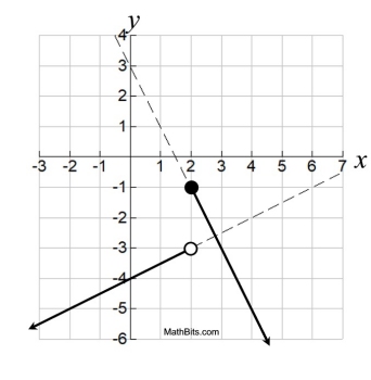
Domain for function f: All real numbers
Range for function f: y < -1
|
Because of the break in the graph, this function is discontinuous.
The graph does pass the Vertical Line Test to be a function.
|
Note: if you are familiar with computer coding,
you can think of piecewise functions as if-else statements (or switch statements).
If a value lies in a certain section of the domain, it is sent to a specific equation, else it is sent to a diffeent equation.
| Piecewise Graphs - on the Graphing Calculator: |
|
For calculator help with Graphing
Piecewise
click here. |
|
|

NOTE: The re-posting of materials (in part or whole) from this site to the Internet
is copyright violation
and is not considered "fair use" for educators. Please read the "Terms of Use". |
|