|
Generic Definition |
In geometry, the term "transformation" refers to manipulating a shape or figure in a coordinate plane, in a effort to change its size, orientation and/or location. The common types of transformations are reflections, translations, rotations and dilations. |
|
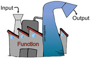
Remember those "function machines" from Algebra 1?
You feed the machine INPUT and it spits out OUTPUT.
For example, if you have a function defined as f (x) = 3x + 1, and you feed it x = 5, the function spits out f (5) = 16.
Well, transformations can be viewed in this same manner. |
|
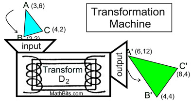 |
Transformations take points in the plane as inputs (pre-image) and give other points as outputs (image).
As such, transformations
behave like "functions". |
|
As you have seen in your previous work with transformations, there are "rules" that define how a transformation takes "input" coordinates (from the pre-image) and creates "output" coordinates (for the image). These applied "rules" may result in translations, reflections, rotations, dilations, or a combination of changes to the original figure.
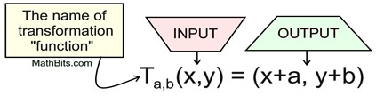
There are a variety of ways to write the "rules" that apply to transformations. The most common form for indicating transformation "rules" is a mapping notation, such as: (x, y)
→ (x + a, y + b).
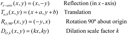
The definitions of the classic transformations may appear in more of a functional notation form:
Notice how this format resembles functional form:
f (x) = 2x + 5
where x is the input and (2x + 5) is the output.
More ways of indicating transformations appear in the section Rigid Transformations.
Transformations can be viewed in terms of functions, where the inputs and outputs are points in the coordinate plane, rather than simply numerical values. We can adjust our definition of "transformations" to reflect the resemblance to functions.
|
Function Based |
A transformation is a geometric function whose domain takes points in the plane as input, and maps them to its range as output. The domain (or input) is called the pre-image . The range (or output) is called the image. |
|

NOTE: The re-posting of materials (in part or whole) from this site to the Internet
is copyright violation
and is not considered "fair use" for educators. Please read the "Terms of Use". |
|
|