Sampling Variability:
| In a real world problem, the statistical information relating to large populations (called parameters) is unknown. Random samples from these large populations are used to estimate information about the population parameters. The term "sampling variability" refers to the fact that the statistical information from a sample (called a statistic) will vary as the random sampling is repeated. Sampling variability will decrease as the sample size increases. |
A parameter is a fixed number that describes a population, such as a percentage, proportion, mean, or standard deviation. In reality, we do not know these numbers because we cannot examine the entire population.
A statistic is a known number that describes a sample, but it can change from sample to sample. |
|
Samplings vary because each sample is based upon a different set of the population. |
When using samples from a large population to determine information about the population parameters, the samples must be randomly chosen, must be of the same size (not smaller than 30), and the more samples that are used, the more reliable the information gathered will be.

Distributions:
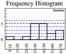
A distribution of statistical data is a listing showing all the possible values (or intervals) of the data and how often they occur. Histograms are a common example of a frequency distribution.
Data set: {9, 25, 30, 31, 34, 36, 37, 42, 45, 47, 49, 43, 55, 58, 61, 63, 67} |
|
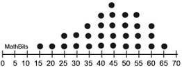
A distribution of a sample is a listing showing each data point in the sample. Sometimes these are referred to as sample distributions (which are NOT sampling distributions). A dot plot may be used to display the distribution of a sample.
Data set: {15, 20, 25, 25, 30, 30, 35, 35, 35, 40, 40, 40, 40, 45, 45, 45, 45, 45, 50, 50, 50, 50, 55, 55, 55, 55, 60, 60, 60, 65} |
|
| A population distribution shows every single possible data point in the population. In most large statistical studies, it is unlikely that the researcher will have access to every single data value in a population. For example, it would not be possible to locate every living gannet (seabird) to measure its wingspan. |
|
Sampling Distribution Models:
Since it is not practical to survey every member of a very large population, statisticians obtain samples of the population, and based upon the characteristics of these samples, they make estimates about the characteristics of the entire population. The more samples that are investigated, the more the observed characteristics will realistically represent the population. This process of inferring population information based upon sample information is called statistical inference.
When dealing with a large number of samples (of the same size) that yield different results for a specific statistic (such as  ), statisticians need to determine which of the samples' results will be the "best" choice to represent the population. This choice is determined by examining all of the possible samples (of the same size) for a specific statistic (such as ) and calculating the average (mean) of that statistic (). In this way, the best "estimate" of the true population parameter will be discovered. This modeling process is a Sampling Distribution of the Sample Means. ), statisticians need to determine which of the samples' results will be the "best" choice to represent the population. This choice is determined by examining all of the possible samples (of the same size) for a specific statistic (such as ) and calculating the average (mean) of that statistic (). In this way, the best "estimate" of the true population parameter will be discovered. This modeling process is a Sampling Distribution of the Sample Means.
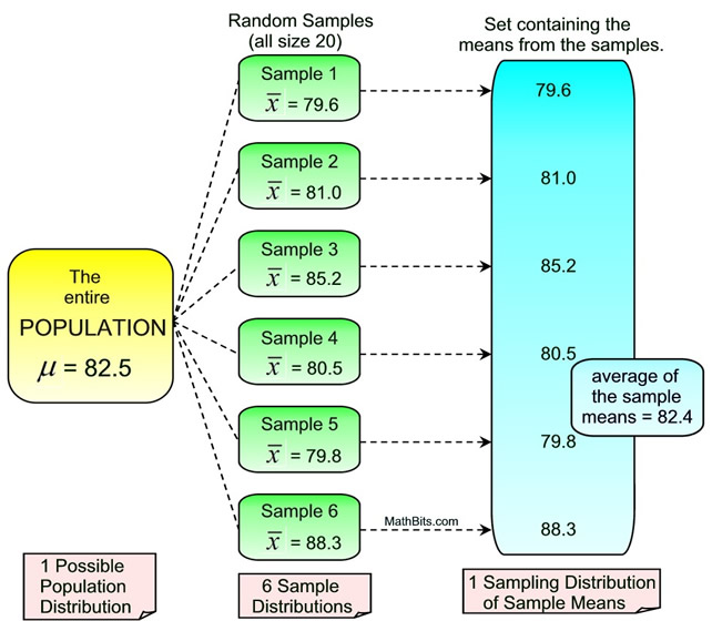
A sampling distribution is the probability distribution of a sample statistic that is formed when samples of size n are repeatedly taken from a population. If the sample statistic is the sample mean, then the distribution is called the sampling distribution of sample means. |
In an attempt to obtain this "best" choice of a statistic, a graph may be prepared to visualize what is happening with that statistic in relation to all of the samples. A dot plot or a histogram is commonly used.
| For example, if we are trying to determine the percentage of Americans that believe in some form of life on other planets, we may obtain 100 sample groups randomly chosen with 50 people in each group. The proportion of people believing in life on other planets from each sample group (19/50, 21/50, 32/50. etc) is determined and graphed. Each dot represents the proportion of people from a sample group of 50 people believing in life on other planets. |
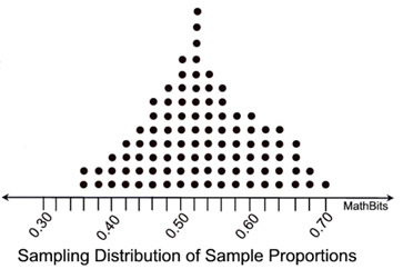 |
The dot plot shows how the proportions from the 100 samples are distributed, and is labeled as the "Sampling Distribution of Sample Proportions". The "mean (average)" of these 100 proportions is used as an estimate of the true proportion for the entire population (all Americans).
In the "life on other planets" example shown above, if we were able to obtain ALL possible samples of size 50 from the population of all Americans, we would be able to state that the mean (average) of ALL of the sampling proportions will be EQUAL to the population proportion.
If you are working with ALL possible samples of a given size, the average of the sampling distribution of the sample statistic (mean or proportion), will be EQUAL to the value of the coordinating population parameter.
If you do not have EVERY possible sample of a given size, you will only have an ESTIMATE of the population parameter. |
In reality, it is usually not possible to obtain ALL possible samples of a given size of a particular population. So, the mean (average) of the "sampling distribution of the sample proportions" will be a good ESTIMATE of the population proportion, and it will get closer and closer to the true population proportion as the sample size is increased. It will, however, most likely not be the "true" population proportion (unless EVERY possible sample of a given size is used.)
In some studies, it is not possible, or practical, to obtain multiple samples of a population. By using simulations, statisticians can quickly create the results from a large number of random sample sets without actually obtaining and examining the sample sets. See how to create a simulation of a sampling distribution on the TI-84+ family of calculators.
 |
Note: Did you notice how the sampling distribution has the appearance of a normal distribution? A theorem, called the Central Limit Theorem, tells us that the sampling distribution of any statistic will be normal, or nearly normal, if the sample size is large enough. As the sample size increases (approaches infinity), we get closer to a true normal distribution. This theorem is true even when the original population is not normally distributed.
|
|
Consider this comparison of "terms" in relation to population, sample, and sampling distribution:
Population: All seniors in the Liverpool High School (N)
Population parameter: Average "grade point average" (GPA) of seniors (μ)
Sample: Students in one senior only class (n)
Sample mean: Average GPA of seniors in that one class ()
Sampling distribution: Distribution of average GPAs from all senior classes (of the same size) surveyed. |
|